Is Today a Good Day to Sell Coffee?

A Beginner’s Guide to Decision Trees

Aug 14, 2025

You’ve got a unique startup idea: a “Portable Coffee Shop” franchise.

What sets your franchise apart is its smart weather-based sales prediction system. Your unique value proposition? Franchisees can check whether today is an optimal day (if you sell on this day, you're set for the month 😂) to set up shop outdoors. If the forecast isn’t favorable, they can take the day off. No wasted effort!

Now it’s time for the next step:
Build an app that predicts whether today is a good day to sell coffee outside.

Example is simple enough, right? 😂 After all, you’re not building the next ChatGPT, just trying to figure out if the weather says “sell” or “do not sell”

To get started, you look at historical data. After squinting at it long enough (and maybe one too many cups of coffee), you spot a pattern: when it’s sunny and the temperature is mild, it’s time to sell!

Here’s what your dataset looks like for the past five days:

data = [ 
  {"Outlook": "Sunny", "Temperature": "Hot", "Sell": "No"},
  {"Outlook": "Sunny", "Temperature": "Mild", "Sell": "Yes"},
  {"Outlook": "Rainy", "Temperature": "Cool", "Sell": "Yes"},
  {"Outlook": "Overcast", "Temperature": "Hot", "Sell": "Yes"},
  {"Outlook": "Rainy", "Temperature": "Mild", "Sell": "No"}
]

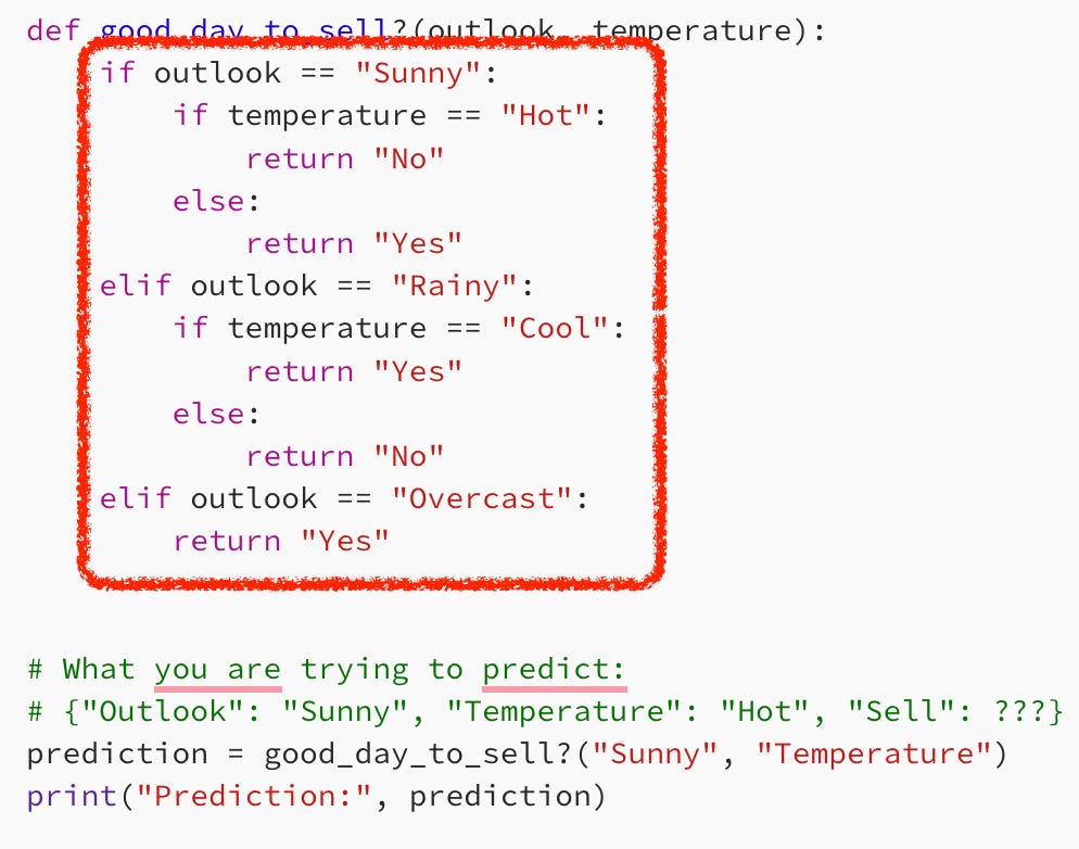
If you’ve been developing apps for a long time like me, you’ll probably think of something like this immediately:

def is_good_day_to_sell(outlook, temperature):
    if outlook == "Sunny":
        if temperature == "Hot":
            return "No"
        else:
            return "Yes"
    elif outlook == "Rainy":
        if temperature == "Cool":
            return "Yes"
        else:
            return "No"
    elif outlook == "Overcast":
        return "Yes"


# What you are trying to predict:
# {"Outlook": "Sunny", "Temperature": "Hot", "Sell": ???}
prediction = is_good_day_to_sell("Sunny", "Hot")
print("Prediction:", prediction)

This function is_good_day_to_sell works! As long as the world never changes. It’s hardcoded based on the exact patterns you’ve seen so far. So if the input is familiar, it gives the correct answer.

But the moment a new combination shows up like this:

{"Outlook": "Sunny", "Temperature": "Cool", "Sell": "???" }

Should it return “Yes” or “No”?

Do you need to add more logical conditions? More “if”, “else”, or “loops”?

What you need is a function that can be trained to see new patterns and then predict. How do you do this?

To truly make your app smarter, you need to allow it to learn from data and adapt to new situations.

You are now leaving the realm of rule-based deterministic programming to data-driven statistical learning (machine learning).

Yes, it’s time for machine learning.

You’ve done your research, and you’ve settled on creating a simple Decision Tree for the app.

P.S. This is a simplified example, not exactly ready to run your coffee empire… but we’ll get there ☕

What’s a decision tree?

A decision tree is like a flowchart that helps you make a decision step-by-step. At each step (called a “node”), the computer asks a yes/no or greater/less than question about a feature (or attribute) of the data.

At the end of the path (a “leaf”), the tree gives you a prediction, like a category or a value.

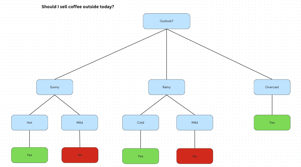
When you look at the definition and image of a decision tree, you might wonder: Couldn’t this just be done with a few logical conditions?

But this brings us back to a key idea, we need algorithms that can learn from data and adapt to new situations. A decision tree isn’t static; it must grow and be pruned dynamically based on the data.

So, as I understand it, we are building a function that generates a function to predict for each new dataset.

So, the real question becomes: How do we build such a tree from data?

To do that, there are two key mathematical concepts you need to understand: Entropy and Information Gain.

No worries, we’ll walk through them step by step. We won’t dive into the formal math proofs, but we will focus on how to translate the equations into code.

Mathematical Concepts

1. Entropy

What is Entropy?
It’s the measure of how much impurity or uncertainty in a dataset.

If all examples in a dataset belong to the same class, the entropy is 0 (pure).
If the examples are equally mixed (e.g., 50% “Yes”, 50% “No”), the entropy is maximum (e.g., in most examples I found, they are 1 or 0).

Yep, the concept is too abstract.

So, let’s apply it to your dataset for some context:

data = [ 
  {"Outlook": "Sunny", "Temperature": "Hot", "Sell": "No"},
  {"Outlook": "Sunny", "Temperature": "Mild", "Sell": "Yes"},
  {"Outlook": "Rainy", "Temperature": "Cool", "Sell": "Yes"},
  {"Outlook": "Overcast", "Temperature": "Hot", "Sell": "Yes"},
  {"Outlook": "Rainy", "Temperature": "Mild", "Sell": "No"}
]

Let’s calculate entropy for the target attribute (What we want to predict): “Sell”

Total examples: 5
“Yes”: 3
“No”: 2

So:

Substituting the values for the Entropy formula we get:

✅ Entropy = 0.971 bits (Entropy for target attribute “Sell”)

You’ve learned the math, now you need to map it to code:

from collections import Counter
import math

# --- Entropy Calculation Function ---
def entropy(data, target):
    # Count the occurrences of each class label in the target attribute
    # For example, in the "Sell" column, we count how many times 
    # "Yes" and "No" appear
    counts = Counter(row[target] for row in data)

    # Total number of examples in the dataset
    total = len(data)

    # Apply the entropy formula:
    # E(S) = -∑ (p_i * log2(p_i)) for each class i
    # Where p_i is the proportion of class i in the dataset
    return -sum((count / total) * math.log2(count / total) for count in counts.values())

# ------------------------------------
# 🧠 Let’s Apply It to Your Dataset
dataset = [
    {"Outlook": "Sunny", "Temperature": "Hot", "Sell": "No"},
    {"Outlook": "Sunny", "Temperature": "Mild", "Sell": "Yes"},
    {"Outlook": "Rainy", "Temperature": "Cool", "Sell": "Yes"},
    {"Outlook": "Overcast", "Temperature": "Hot", "Sell": "Yes"},
    {"Outlook": "Rainy", "Temperature": "Mild", "Sell": "No"}
]

# We want to calculate the entropy of the target attribute: "Sell"
# Breakdown:
# Total examples = 5
# "Yes" = 3 → p_Yes = 3/5 = 0.6
# "No"  = 2 → p_No  = 2/5 = 0.4

# Entropy formula:
# E(S) = -[0.6 * log2(0.6) + 0.4 * log2(0.4)]
#      ≈ -[0.6 * (-0.737) + 0.4 * (-1.322)]
#      ≈ 0.971 bits

# ✅ Now let's calculate it using our function:
result = entropy(dataset, "Sell")
print("Entropy of 'Sell':", round(result, 3))  # Expected output: 0.971

2. Information Gain

Information Gain (IG) measures how much uncertainty (entropy) is reduced after splitting the data based on an attribute.

Again, let’s make this definition more understandable with examples on your data:

dataset = [
    {"Outlook": "Sunny", "Temperature": "Hot", "Sell": "No"},
    {"Outlook": "Sunny", "Temperature": "Mild", "Sell": "Yes"},
    {"Outlook": "Rainy", "Temperature": "Cool", "Sell": "Yes"},
    {"Outlook": "Overcast", "Temperature": "Hot", "Sell": "Yes"},
    {"Outlook": "Rainy", "Temperature": "Mild", "Sell": "No"}
]

Let’s compute the information gain of the attribute: “Outlook”

Step 1: Group by “Outlook”

+----------+---------+-------------+
| Outlook  | Subset  | Sell values |
+----------+---------+-------------+
| Sunny    | Row 1,2 | No, Yes     |
| Rainy    | Row 3,5 | Yes, No     |
| Overcast | Row 4   | Yes         |
+----------+---------+-------------+

Step 2: Compute the entropy of each subset

Outlook = Sunny (2 items)

“No”: 1
“Yes”: 1

Outlook = Rainy (2 items)

“Yes”: 1
“No”: 1

Outlook = Overcast (1 item)

“Yes”: 1

✅ Information Gain for “Outlook” = 0.171

You’ve learned the math, now you need to map it to code. Note that this uses the entropy function we’ve discussed above:

def information_gain(data, feature, target):
    # Step 1️⃣: Compute the total entropy of the entire dataset using
    # only the target class
    # This corresponds to: E(S) = 0.971 in your example
    total_entropy = entropy(data, target)

    # Step 2️⃣: Get all unique values of the attribute 
    # we're evaluating (e.g., Outlook = Sunny, Rainy, Overcast)
    values = set(row[feature] for row in data)

    # Step 3️⃣: Initialize the weighted sum of entropies after the split
    weighted_entropy = 0.0

    # Step 4️⃣: For each value (e.g., "Sunny"), compute:
    for value in values:
        # a. Subset the dataset where feature == value 
        # (e.g., Outlook == Sunny)
        subset = [row for row in data if row[feature] == value]

        # b. Calculate the proportion of the subset relative 
        # to the total data
        weight = len(subset) / len(data)

        # c. Compute entropy of the subset (based only on 
        # the target variable "Sell")
        subset_entropy = entropy(subset, target)

        # d. Add this weighted entropy to the total
        weighted_entropy += weight * subset_entropy

    # Step 5️⃣: Subtract weighted entropy from total entropy to 
    # get Information Gain
    return total_entropy - weighted_entropy

    # 🧠 Let's Apply Information Gain to "Outlook"
    # Total entropy of "Sell" was calculated before: ≈ 0.971

    # We'll now compute the weighted entropy after splitting by "Outlook":
    # Outlook has 3 unique values: Sunny, Rainy, Overcast

    # 🌤 Sunny subset:
    #   [{"Sunny", "Hot", "No"}, {"Sunny", "Mild", "Yes"}]
    #   - 2 samples: 1 Yes, 1 No → entropy = 1.0
    #   - weight = 2/5 = 0.4
    #   - weighted entropy = 0.4 × 1.0 = 0.4

    # 🌧 Rainy subset:
    #   [{"Rainy", "Cool", "Yes"}, {"Rainy", "Mild", "No"}]
    #   - 2 samples: 1 Yes, 1 No → entropy = 1.0
    #   - weight = 2/5 = 0.4
    #   - weighted entropy = 0.4 × 1.0 = 0.4

    # ☁️ Overcast subset:
    #   [{"Overcast", "Hot", "Yes"}]
    #   - 1 sample: 1 Yes → entropy = 0
    #   - weight = 1/5 = 0.2
    #   - weighted entropy = 0.2 × 0 = 0.0

    # 🔄 Total Weighted Entropy = 0.4 + 0.4 + 0.0 = 0.8

    # ✅ Information Gain = Total Entropy - Weighted Entropy
    #                    = 0.971 - 0.8
    #                    = 0.171

    # Let's run the function:
    gain_outlook = information_gain(dataset, "Outlook", "Sell")
    print("Information Gain for 'Outlook':", round(gain_outlook, 3))  
    # Expected: 0.171

In decision trees, it is used to select the best attribute to split on, the one that provides the highest IG. This will become clearer later once I use the information gain function.

Building the Tree

We’ve built the functions for Entropy and Information Gain; the next step is to create a function that builds the tree.

Here’s the step on how we build the tree:

Calculate Information Gain for “Outlook” and “Temperature”.
Select the feature with higher Information Gain (likely “Outlook”)
Split the data based on Outlook values (Sunny, Rainy, Overcast)
Recursively build subtrees for each branch.

Here’s the code for that:

def build_tree(data, features, target):
    
    # Extract all target labels from the current data subset
    # Example: if target="Sell", labels = ["No", "Yes", "Yes", "Yes", "No"]
    labels = [row[target] for row in data]
    
    # BASE CASE 1: Pure Node (All labels are the same)
    # If all instances have the same target label, create a leaf node
    # Example: labels = ["Yes", "Yes", "Yes"] → return "Yes"
    if labels.count(labels[0]) == len(labels):
        return labels[0]
    
    # BASE CASE 2: No Features Left (Feature exhaustion)
    # If we've used all features but still have mixed labels,
    # return the most common label (majority vote)
    # Example: labels = ["No", "Yes", "No"] → return "No" (majority)
    if not features:
        return Counter(labels).most_common(1)[0][0]

    # RECURSIVE CASE: Feature Selection and Splitting
    
    # Step 1: Calculate information gain for each remaining feature
    # Dictionary comprehension creates: {"Outlook": 0.25, "Temperature": 0.15}
    gains = {feature: information_gain(data, feature, target) for feature in features}
    
    # Step 2: Select the feature with the highest information gain
    # Uses max() with key=gains.get to find the key with maximum value
    best_feature = max(gains, key=gains.get)

    # Step 3: Create the tree node structure
    # Creates a dictionary where the key is the splitting feature
    # Example: {"Outlook": {}} - empty dict will hold the branches
    tree = {best_feature: {}}
    
    # Step 4: Get all unique values for the chosen feature
    # Example: if best_feature="Outlook", values = {"Sunny", "Rainy", "Overcast"}
    values = set(row[best_feature] for row in data)
    
    # Step 5: For each unique value, create a branch by recursive splitting
    for value in values:
        # Filter data to only include rows with this feature value
        # Example: subset for "Sunny" = all rows where Outlook="Sunny"
        subset = [row for row in data if row[best_feature] == value]
        
        # Recursively build a subtree for this subset using remaining features
        # Remove the current feature from available features to prevent reuse
        # Example: if we used "Outlook", remaining features = ["Temperature"]
        subtree = build_tree(subset, [f for f in features if f != best_feature], target)
        
        # Attach the returned subtree to the current tree node
        # Example: tree["Outlook"]["Sunny"] = {subtree for sunny conditions}
        tree[best_feature][value] = subtree

    # Return the completed tree structure
    # Final structure: 
    # Outlook?
    #   ├── Sunny:
    #   │   └── Temperature?
    #   │       ├── Hot → Yes
    #   │       └── Mild → No
    #   ├── Rainy:
    #   │   └── Temperature?
    #   │       ├── Hot → Yes
    #   │       └── Cool → No
    #   └── Overcast:
    #       └── Temperature?
    #           ├── Hot → No
    #           └── Cool → Yes
    return tree

Updating the function

Based on what we’ve learned, now it’s time to update the is_good_day_to_sell function:

def is_good_day_to_sell(tree, instance):
    """
    Prediction function that traverses a decision tree to make 
    predictions for new instances.Implements the inference/prediction 
    phase of the decision tree algorithm using recursion.
    
    Parameters:
    - tree: The trained decision tree structure (nested dictionaries) 
            created by build_tree
    - instance: A dictionary representing a new data point to classify 
                (e.g., {"Outlook": "Sunny", "Temperature": "Mild"})
    
    Returns:
    - The classification label (e.g., "Yes" or "No")
    
    Example traversal for instance {"Outlook": "Sunny", "Temperature": "Mild"}:
    Step 1: tree is dict, feature="Outlook", value="Sunny" 
    Step 2: subtree = tree["Outlook"]["Sunny"] (Temperature subtree)
    Step 3: Recursive call with Temperature subtree
    Step 4: tree is dict, feature="Temperature", value="Mild"
    Step 5: subtree = "Yes" (leaf node)
    Step 6: tree is not dict, return "Yes"
    """
    
    # BASE CASE - Leaf Node: If tree is not a dictionary, 
    # we've reached a leaf node containing the final 
    # prediction/classification label
    if not isinstance(tree, dict):
        return tree
    
    # Get the splitting feature from the current tree node
    # Since each tree node is a dictionary with one key (the splitting feature),
    # this extracts that feature name. Example: {"Outlook": {...}} → feature = "Outlook"
    feature = next(iter(tree))
    
    # Look up the value of the current feature in the instance being classified
    # Example: If feature="Outlook" and instance={"Outlook": "Sunny", ...}, then value="Sunny"
    value = instance.get(feature)
    
    # Navigate to the subtree corresponding to the instance's feature value
    # Example: tree["Outlook"].get("Sunny") returns the subtree for sunny conditions
    subtree = tree[feature].get(value)
    
    # RECURSIVE CASE: Continue traversing down the tree with the selected subtree
    # This follows the decision path through the tree based on the instance's feature values
    # until reaching a leaf node containing the final prediction
    return is_good_day_to_sell(subtree, instance)

Evaluation

This wouldn't feel like an AI blog if we didn’t compare our new algorithm to the previous one. How does our new algorithm compared to our original one?

Here’s how the evaluation was done:

from build_tree import build_tree
from is_good_day_to_sell import is_good_day_to_sell
from static_tree_predict import static_tree_predict

# --- Dataset ---
dataset = [
    {"Outlook": "Sunny", "Temperature": "Hot", "Sell": "No"},
    {"Outlook": "Sunny", "Temperature": "Mild", "Sell": "Yes"},
    {"Outlook": "Rainy", "Temperature": "Cool", "Sell": "Yes"},
    {"Outlook": "Overcast", "Temperature": "Hot", "Sell": "Yes"},
    {"Outlook": "Rainy", "Temperature": "Mild", "Sell": "No"}
]

features = ["Outlook", "Temperature"]
target = "Sell"

# Complex dataset
complex_dataset = [
    {"Outlook": "Sunny", "Temperature": "Hot", "Sell": "Yes"},     # contradiction to static
    {"Outlook": "Sunny", "Temperature": "Cool", "Sell": "No"},     # contradiction
    {"Outlook": "Sunny", "Temperature": "Mild", "Sell": "Yes"},
    {"Outlook": "Rainy", "Temperature": "Hot", "Sell": "Yes"},     # unseen combo
    {"Outlook": "Rainy", "Temperature": "Cool", "Sell": "No"},     # contradiction
    {"Outlook": "Rainy", "Temperature": "Mild", "Sell": "Yes"},    # flipped
    {"Outlook": "Overcast", "Temperature": "Hot", "Sell": "Yes"},
    {"Outlook": "Overcast", "Temperature": "Cool", "Sell": "No"},  # exception
    {"Outlook": "Overcast", "Temperature": "Mild", "Sell": "Yes"},
    {"Outlook": "Sunny", "Temperature": "Hot", "Sell": "Yes"},     # repeat for reinforcement
]

# Much more challenging dataset that exposes static tree limitations
challenging_dataset = [
    # Sunny days - Static tree says Hot=No, others=Yes
    # Let's make the pattern more complex: depends on both features together
    {"Outlook": "Sunny", "Temperature": "Hot", "Sell": "Yes"},      # Static: No, should be Yes
    {"Outlook": "Sunny", "Temperature": "Hot", "Sell": "Yes"},      # Reinforce pattern
    {"Outlook": "Sunny", "Temperature": "Hot", "Sell": "Yes"},      # Static gets this wrong
    {"Outlook": "Sunny", "Temperature": "Mild", "Sell": "No"},      # Static: Yes, should be No
    {"Outlook": "Sunny", "Temperature": "Mild", "Sell": "No"},      # Reinforce
    {"Outlook": "Sunny", "Temperature": "Cool", "Sell": "Yes"},     # Static: Yes, correct by luck
    {"Outlook": "Sunny", "Temperature": "Cool", "Sell": "Yes"},
    
    # Rainy days - Static tree says Cool=Yes, others=No  
    # Let's completely flip this pattern
    {"Outlook": "Rainy", "Temperature": "Cool", "Sell": "No"},      # Static: Yes, should be No
    {"Outlook": "Rainy", "Temperature": "Cool", "Sell": "No"},      # Reinforce
    {"Outlook": "Rainy", "Temperature": "Cool", "Sell": "No"},      # Static gets this wrong
    {"Outlook": "Rainy", "Temperature": "Mild", "Sell": "Yes"},     # Static: No, should be Yes
    {"Outlook": "Rainy", "Temperature": "Mild", "Sell": "Yes"},     # Reinforce
    {"Outlook": "Rainy", "Temperature": "Hot", "Sell": "Yes"},      # Static: No, should be Yes
    {"Outlook": "Rainy", "Temperature": "Hot", "Sell": "Yes"},      # Reinforce
    
    # Overcast days - Static tree always says Yes
    # Let's make it depend on temperature in a different way
    {"Outlook": "Overcast", "Temperature": "Hot", "Sell": "No"},    # Static: Yes, should be No
    {"Outlook": "Overcast", "Temperature": "Hot", "Sell": "No"},    # Reinforce
    {"Outlook": "Overcast", "Temperature": "Hot", "Sell": "No"},    # Static gets this wrong
    {"Outlook": "Overcast", "Temperature": "Mild", "Sell": "Yes"},  # Static: Yes, correct by luck
    {"Outlook": "Overcast", "Temperature": "Mild", "Sell": "Yes"},
    {"Outlook": "Overcast", "Temperature": "Cool", "Sell": "Yes"},  # Static: Yes, correct by luck
    {"Outlook": "Overcast", "Temperature": "Cool", "Sell": "Yes"},
    
    # Additional edge cases to really challenge the static tree
    {"Outlook": "Sunny", "Temperature": "Hot", "Sell": "Yes"},      # More evidence against static
    {"Outlook": "Rainy", "Temperature": "Cool", "Sell": "No"},      # More evidence against static
    {"Outlook": "Overcast", "Temperature": "Hot", "Sell": "No"},    # More evidence against static
]

# Extreme challenge dataset - completely opposite to static tree assumptions
extreme_dataset = [
    # Make the static tree fail catastrophically
    # Sunny + Hot should be Yes (static says No)
    {"Outlook": "Sunny", "Temperature": "Hot", "Sell": "Yes"},
    {"Outlook": "Sunny", "Temperature": "Hot", "Sell": "Yes"},
    {"Outlook": "Sunny", "Temperature": "Hot", "Sell": "Yes"},
    {"Outlook": "Sunny", "Temperature": "Hot", "Sell": "Yes"},
    {"Outlook": "Sunny", "Temperature": "Hot", "Sell": "Yes"},
    
    # Sunny + others should be No (static says Yes)
    {"Outlook": "Sunny", "Temperature": "Mild", "Sell": "No"},
    {"Outlook": "Sunny", "Temperature": "Mild", "Sell": "No"},
    {"Outlook": "Sunny", "Temperature": "Cool", "Sell": "No"},
    {"Outlook": "Sunny", "Temperature": "Cool", "Sell": "No"},
    
    # Rainy + Cool should be No (static says Yes)
    {"Outlook": "Rainy", "Temperature": "Cool", "Sell": "No"},
    {"Outlook": "Rainy", "Temperature": "Cool", "Sell": "No"},
    {"Outlook": "Rainy", "Temperature": "Cool", "Sell": "No"},
    {"Outlook": "Rainy", "Temperature": "Cool", "Sell": "No"},
    
    # Rainy + others should be Yes (static says No)
    {"Outlook": "Rainy", "Temperature": "Mild", "Sell": "Yes"},
    {"Outlook": "Rainy", "Temperature": "Mild", "Sell": "Yes"},
    {"Outlook": "Rainy", "Temperature": "Hot", "Sell": "Yes"},
    {"Outlook": "Rainy", "Temperature": "Hot", "Sell": "Yes"},
    
    # Overcast should sometimes be No (static always says Yes)
    {"Outlook": "Overcast", "Temperature": "Hot", "Sell": "No"},
    {"Outlook": "Overcast", "Temperature": "Hot", "Sell": "No"},
    {"Outlook": "Overcast", "Temperature": "Hot", "Sell": "No"},
    {"Outlook": "Overcast", "Temperature": "Mild", "Sell": "Yes"},
    {"Outlook": "Overcast", "Temperature": "Cool", "Sell": "Yes"},
]

def compare_predictions(tree, dataset, title=""):
    """Compare predictions between static tree and ML tree."""
    print(f"\n📊 {title}")
    print(f"{'Outlook':<10} {'Temp':<10} {'Actual':<7} {'Static':<8} {'ML Tree':<8} {'Match?'}")
    for row in dataset:
        actual = row["Sell"]
        static_pred = static_tree_predict(row)
        ml_pred = is_good_day_to_sell(tree, row)
        match = "✅" if static_pred == ml_pred else "❌"
        print(f"{row['Outlook']:<10} {row['Temperature']:<10} {actual:<7} {static_pred:<8} {ml_pred:<8} {match}")

def compute_accuracy(predict_fn, data, target):
    """Compute accuracy of a prediction function on a dataset."""
    correct = 0
    for row in data:
        if predict_fn(row) == row[target]:
            correct += 1
    return correct / len(data)

def detailed_comparison(tree, dataset, title=""):
    """Provide detailed analysis of where static vs ML tree differ"""
    print(f"\n🔍 DETAILED ANALYSIS: {title}")
    print("="*80)
    
    static_correct = 0
    ml_correct = 0
    both_correct = 0
    both_wrong = 0
    static_better = 0
    ml_better = 0
    
    disagreements = []
    
    for row in dataset:
        actual = row["Sell"]
        static_pred = static_tree_predict(row)
        ml_pred = is_good_day_to_sell(tree, row)
        
        static_right = static_pred == actual
        ml_right = ml_pred == actual
        
        if static_right:
            static_correct += 1
        if ml_right:
            ml_correct += 1
            
        if static_right and ml_right:
            both_correct += 1
        elif not static_right and not ml_right:
            both_wrong += 1
        elif static_right and not ml_right:
            static_better += 1
        elif not static_right and ml_right:
            ml_better += 1
            
        if static_pred != ml_pred:
            disagreements.append({
                'case': f"{row['Outlook']}-{row['Temperature']}",
                'actual': actual,
                'static': static_pred,
                'ml': ml_pred,
                'static_right': static_right,
                'ml_right': ml_right
            })
    
    total = len(dataset)
    print(f"📈 ACCURACY COMPARISON:")
    print(f"   Static Tree:  {static_correct:2d}/{total} = {static_correct/total:.1%}")
    print(f"   ML Tree:      {ml_correct:2d}/{total} = {ml_correct/total:.1%}")
    print(f"   Improvement:  {ml_correct-static_correct:+2d} predictions = {(ml_correct-static_correct)/total:+.1%}")
    
    print(f"\n🎯 AGREEMENT ANALYSIS:")
    print(f"   Both Correct: {both_correct:2d}/{total} = {both_correct/total:.1%}")
    print(f"   Both Wrong:   {both_wrong:2d}/{total} = {both_wrong/total:.1%}")
    print(f"   Static Better:{static_better:2d}/{total} = {static_better/total:.1%}")
    print(f"   ML Better:    {ml_better:2d}/{total} = {ml_better/total:.1%}")
    
    if disagreements:
        print(f"\n⚔️  DISAGREEMENTS ({len(disagreements)} cases):")
        print(f"{'Case':<15} {'Actual':<7} {'Static':<7} {'ML':<7} {'Winner'}")
        print("-" * 50)
        for d in disagreements:
            if d['static_right'] and not d['ml_right']:
                winner = "Static ✅"
            elif not d['static_right'] and d['ml_right']:
                winner = "ML ✅"
            elif not d['static_right'] and not d['ml_right']:
                winner = "Both ❌"
            else:
                winner = "Both ✅"
            print(f"{d['case']:<15} {d['actual']:<7} {d['static']:<7} {d['ml']:<7} {winner}")
    
    return {
        'static_accuracy': static_correct/total,
        'ml_accuracy': ml_correct/total,
        'improvement': (ml_correct-static_correct)/total,
        'disagreements': len(disagreements)
    }

if __name__ == "__main__":
    # Train the tree on original dataset
    tree = build_tree(dataset, features, target)
    print("🌳 Learned Tree Structure:")
    print(tree)

    # Simple demo
    print("\n" + "="*50)
    print("🚀 SIMPLE DEMO")
    print("="*50)
    test_instance = {"Outlook": "Sunny", "Temperature": "Mild"}
    print("Prediction for", test_instance, "->", is_good_day_to_sell(tree, test_instance))
    
    print("\n" + "="*100)
    print("🧪 TESTING DIFFERENT DATASETS TO EXPOSE STATIC TREE LIMITATIONS")
    print("="*100)

    # Test 1: Original simple data
    print("\n" + "🔹"*50)
    print("TEST 1: Original Training Data (should work well for both)")
    detailed_comparison(tree, dataset, "Original Training Data")

    # Test 2: Basic complex data  
    print("\n" + "🔹"*50)
    print("TEST 2: Basic Complex Data (some contradictions)")
    detailed_comparison(tree, complex_dataset, "Basic Complex Data")

    # Test 3: More challenging data
    print("\n" + "🔹"*50)
    print("TEST 3: Challenging Dataset (systematic patterns opposite to static tree)")
    challenging_tree = build_tree(challenging_dataset, features, target)
    print(f"🌳 New tree learned from challenging data: {challenging_tree}")
    detailed_comparison(challenging_tree, challenging_dataset, "Challenging Dataset")

    # Test 4: Extreme challenge
    print("\n" + "🔹"*50)
    print("TEST 4: Extreme Challenge (completely opposite patterns)")
    extreme_tree = build_tree(extreme_dataset, features, target)
    print(f"🌳 New tree learned from extreme data: {extreme_tree}")
    detailed_comparison(extreme_tree, extreme_dataset, "Extreme Challenge Dataset")

This is the result:

See the authentic surprise in my face after running it the nth time. 😂

This isn’t a very sophisticated evaluation, but it will hopefully give you an idea of why the Decision Tree learner is better than the static one. By the way, I’m calling the first version of the “prediction” function as static_tree_predict to distinguish it from the learning one, which is called the is_good_day_to_sell.

The reasoning on how the datasets is “harder” is commented on the code.

✅ Test 1: Original Training Data

+------------+-------------+---------------------------------+
| Metric     | Static Tree | ML Tree                         |
+------------+-------------+---------------------------------+
| Accuracy   | 100%        | 100%                            |
| Improvement| 0%          | —                               |
| Agreement  | Perfect     | Both agreed on every prediction |
+------------+-------------+---------------------------------+

🧪 Test 2: Complex Dataset

+---------------+-------------+-------------------------+
| Metric        | Static Tree | ML Tree                 |
+---------------+-------------+-------------------------+
| Accuracy      | 30%         | 40%                     |
| Improvement   | +10%        | +1 correct prediction   |
| Disagreements | 1 case      | ML better in that case  |
+---------------+-------------+-------------------------+

🔥 Test 3: Challenging Dataset

+---------------+-------------+---------------------------+
| Metric        | Static Tree | ML Tree                   |
+---------------+-------------+---------------------------+
| Accuracy      | 30%         | 40%                       |
| Improvement   | +10%        | +1 correct prediction     |
| Disagreements | 1 case      | ML better in that case    |
+---------------+-------------+---------------------------+

🚨 Test 4: Extreme Challenge Dataset

+---------------+-------------+---------------------------+
| Metric        | Static Tree | ML Tree                   |
+---------------+-------------+---------------------------+
| Accuracy      | 9.1%        | 100%                      |
| Improvement   | +90.9%      | +20 correct predictions   |
| Disagreements | 20 cases    | All won by ML Tree        |
+---------------+-------------+---------------------------+

Observations

The Decision Tree (ML tree), learns from data and adapts well to new patterns, showing significant improvement when the data distribution changes. However, it may fail when trained on flipped or misleading data and then tested on the original, revealing a risk of overfitting.

In contrast, the static tree (original code) relies on hardcoded logic and only performs well under fixed patterns. It fails catastrophically when exposed to unseen or contradictory inputs and cannot update itself without manual reprogramming, making it brittle in dynamic environments.

Conclusion

You’ve built the app ! Now it’s time to launch your startup and chase that unicorn status! 🦄 Go make it happen!

☕ Just a Quick Reality Check

Okay, this whole post is a beginner-friendly crash course in Decision Trees. It’s meant to help you see how machines can learn from patterns, not replace scikit-learn, your favorite ML library, or actual data science best practices.

The code here is more of a proof of concept than something you’d ship to production. No error handling, no fancy pruning, no cross-validation. Just vibes, recursion, and decision-making magic. ✨

Thanks for sticking with me this far! I know it got a bit lengthy. I couldn’t quite trim it down as much as I wanted. As a little reward, here’s a photo of my Dobermann pup, Claude, named after Claude Shannon, the father of information theory (yes, the same one behind Entropy and Information Gain).

Building Apps for Startups with Ademar Tutor

Discussion about this post